Tutorial & Examples
Growing planetary systems with pebble snow.
Download this page as a jupyter notebook.
Users can model planet formation via pebble snow by:
create a
Disk()object (the protoplanetary disk), which predicts the pebble mass flux and flux-averaged Stokes numbercreate a
Seeds()object (the planetesimal seed masses), anduse class function
Seeds.grow()to grow the planetesimals and store outputs as attributes
For a full list of parameters, see the documentation here
Begin by importing:
import thePPOLsCode as plc
import numpy as np
import matplotlib.pyplot as plt
Example 1 - Simple System with Static Snow Line
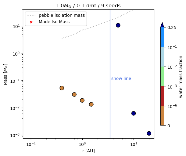
This simple case will create a Disk() around a 1 solar mass star, a
disk mass fraction (dmf) of 0.10 (gas + dust = 10% of stellar mass), and
a snow line set at 3.5 au. By default, alpha = 10^-3 so we do not
include it this time. The second line disk.inspect() is a
convenience function to print basic information about the disk.
disk = plc.Disk(MSol=1.0, dmf=0.1, snowmode=3.5)
disk.inspect() #inspect(plots=True)
Output:
Mstar = 1.0 MSol
Disk mass = 0.100 MSol / 33295 MEarth
Dust mass =  446 MEarth
SigmaGas/Dust at 1 AU = 4382 / 29 [g/cm^2]
Snowline = 3.50 au
disk contains many informative attributes, such as the stellar mass,
disk mass, temperatue profile, and location of the snow line,
e.g. disk.MSol, disk.dmf, disk.snowline_au.
The attributes disk.tgrid and disk.rgrid provide the time and
spatial dimension of the disk in cgs units (seconds and cm).
Next, we create planetesimal seed masses at the location of the solar
system planets, with an initial mass ~Pluto at
\(10^{-3} M_{\oplus}\). We also need to specificy which disk
object the seeds belong to. Finally, exectue seeds.grow() to make
your planetary system:
seeds_au = np.array([0.4, 0.7, 1.0, 1.5, 5, 10, 20, 30, 40]) # locations, au
mass = 1e-3 # Earth masses

seeds = plc.Seeds(disk=disk, seeds_au=seeds_au, mass=mass)
seeds.grow()
A convenience plotting function exists to show the protoplanet masses, water mass fraction, snow line position, and pebble isolation mass:
seeds.gtplot()
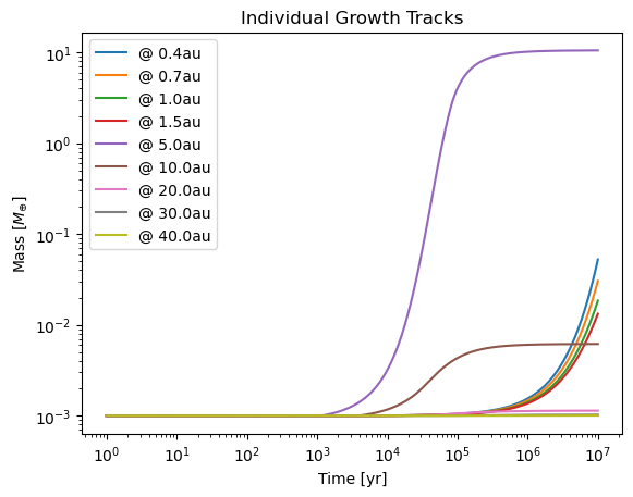
As with Disk, there are many attributes added to the Seeds
object that are recorded and at each time step. By default, growth
proceeds for 10 million years. Thus, growth tracks for each seed mass
can be plotted using:
year = 365.25*24*3600
fig, ax = plt.subplots()
for i, s in enumerate(seeds_au):
    ax.plot(disk.tgrid/year, seeds.cumulmass[i], label='@ {:1.1f}au'.format(s))
ax.set(yscale='log', xscale='log', ylabel='Mass [$M_{\oplus}$]', xlabel='Time [yr]',
      title='Individual Growth Tracks')
ax.legend()
Example 2 - Evolving Snow Line
Let’s spice things up with another example - this time we will grow 80 seeds distributed exponentially from 0.5 to 120 AU, starting from \(10^{-4} M_{\oplus}\), around a 0.5\(M_{\odot}\) star, with an initial total disk mass fraction that is 1% of the stellar mass, and an evolving snow line.
To implement a snow line that is based off disk conditions, and that
evolves as the dust converts into pebbles (see Equation 5 from McCloat
et al. 2025), use snowmode='evol' during Disk() creation:
disk_2 = plc.Disk(MSol=0.5, dmf=0.01, snowmode='evol')
seeds_au_2 = np.geomspace(0.05, 120, 80)
mass_2 = 1e-4
seeds_2 = plc.Seeds(disk=disk_2, seeds_au=seeds_au_2, mass=mass_2)
seeds_2.grow()
seeds_2.gtplot(ylim=[1e-5,1e2], xlim=[0.01,1])
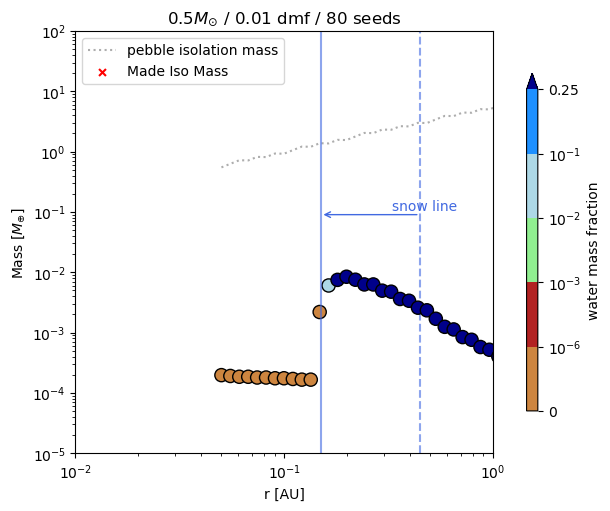
Notice how this time the starting and end locations of the snow line are
marked with the light blue dashed –> solid line. Notice also you can
tweak the figure limits in the call to gtplot().
Example 3 - Explicit Solid Disk Mass & Staggered Formation Time
Some investigators may be interested in setting the solid disk mass
explicitly instead of as a total fraction of the stellar mass. This is
easily accomplished by setting dmf > 1: this will set initial solid
dust mass, in Earth masses. Users can also adjust the dust-gas ratio of
the disk using z0.
To change the introduction time of the seeds into the disk,
i.e. planetesimal seed masses form later at greater distances, use the
Seeds parameter tintro=. We can also set the initial mass of
each planetesimal seed in the same way. Note these arrays need to be the
same length as the location (seeds_au).
In this example, we will set the dust mass to 600 \(M_{\oplus}\), the disk metallicity (dust-gas ratio) to 0.91, and stagger the introduction mass and formation time of the seeds:
disk_3 = plc.Disk(MSol=0.75, dmf=600, z0=0.91, snowmode='temp')

n = 80  # the number of seeds
seeds_au_3 = np.geomspace(0.05, 120, n)
mass_3 = np.geomspace(1e-5, 1e-2, n)
tintro = np.geomspace(1e3, 5e5, n)
seeds_3 = plc.Seeds(disk=disk_3, seeds_au=seeds_au_3, mass=mass_3, tintro=tintro)

seeds_3.grow()
seeds_3.gtplot(ylim=[1e-5,1e2], xlim=[0.01,100])
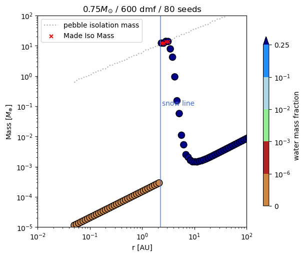
In Example 3 above, we also used snowmode='temp' to flesh out its
capability. In this example, several of the seeds just behind the snow
line grew very efficiently and reached the pebble isolation mass. When
this occurs, they will essentially block the iwnard flow of pebbles
behind them and starve the inner seeds of growth.
Other Parameters
tempmode: temperature, by default, the disk is set with a power law
temperature profile. An alternate temperature profile from Ida et
al. 2016 that accounts for viscous and irradiation heating is also
available. Use tempmode = 'ida2016'.
The main functionality of the PPOLs Model is to enable flexible efficient planetary assembly via pebble snow, tracking the mass and water mass fraction of growing seed masses. Users can change the stellar mass, disk mass, snow line position in a variety of ways. Be sure to explore the docs for all the options and review the published paper McCloat et al. (2025).
Many useful physical parameters are available as attributes in the Disk or Seeds object, and most paramaters are recorded as functions of both radial position (au) and time. Please reach out to spmccloat@gmail.com with questions.